Eigenvector

Properties#

• Only the direction is determined: if $x$ is an eigenvector for $\lambda$, so is $cx$ for every $c \neq 0$, since $A(cx) = cAx = \lambda(cx)$ (MML p. 105). An eigenvector is therefore usually given up to scaling, e.g. normalized to $\|x\| = 1$. Two vectors that point in the same or the opposite direction are called collinear.
• Eigenspaces are subspaces: $E_\lambda$ is the solution set of the homogeneous linear system $(A - \lambda I)x = 0$, so it is the kernel of $A - \lambda I$. Every linear combination of eigenvectors for the same $\lambda$ is again in $E_\lambda$.
• Multiplicities: $1 \le \dim E_\lambda \le$ algebraic multiplicity of $\lambda$ (MML p. 108).
• $A$ and $A^\top$ have the same eigenvalues, but in general not the same eigenvectors.

ProofProof (beyond the lecture)

Induction on $k$; $k = 1$ holds since $x_1 \neq 0$. Suppose $\sum_{i=1}^k c_i x_i = 0$. Applying $A$ gives $\sum_i c_i\lambda_i x_i = 0$, and multiplying the first equation by $\lambda_k$ gives $\sum_i c_i\lambda_k x_i = 0$. Subtracting: $\sum_{i=1}^{k-1} c_i(\lambda_i - \lambda_k)x_i = 0$. By induction $c_i(\lambda_i - \lambda_k) = 0$, and since $\lambda_i \neq \lambda_k$, $c_i = 0$ for $i < k$. Then $c_k x_k = 0$ gives $c_k = 0$.

A matrix with fewer than $n$ linearly independent eigenvectors is defective (MML Def. 4.13). It has an eigenvalue whose geometric multiplicity is smaller than its algebraic multiplicity.

ProofWhy

$AP = [Ap_1, \dots, Ap_n]$ and $PD = [\lambda_1 p_1, \dots, \lambda_n p_n]$, so $AP = PD$ iff $Ap_i = \lambda_i p_i$ for all $i$. $P$ is invertible iff its columns form a basis, and then $AP = PD \iff A = PDP^{-1}$ (MML pp. 116–117).

Read $A = PDP^{-1}$ from right to left: $P^{-1}$ changes to coordinates in the eigenbasis, $D$ scales each coordinate by its eigenvalue, and $P$ changes back. Powers become easy: $A^k = PD^kP^{-1}$.

Eigenvectors of a symmetric matrix for different eigenvalues are automatically orthogonal. Within one eigenspace of dimension $> 1$ an orthonormal basis can be chosen with Gram–Schmidt (MML Example 4.8). This is the decomposition behind the eigenvalue test for positive semidefinite matrices.

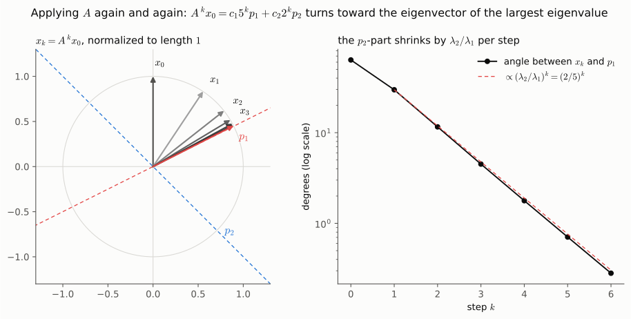
Power iteration (MML Example 4.9, PageRank): if $A$ has an eigenvalue $\lambda_1$ with $|\lambda_1|$ strictly larger than all others, then the directions of $x, Ax, A^2x, \dots$ converge to the eigenvector of $\lambda_1$ for almost every start vector $x$. See Intuition for why.

Example#

Intuition#

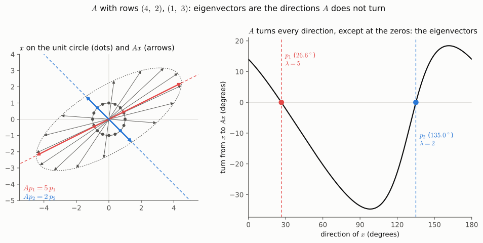
A linear map usually turns a vector as well as stretching it. Left: the unit vectors $x$ (dots) and their images $Ax$ (arrows) for $A = \begin{pmatrix} 4 & 2 \\ 1 & 3 \end{pmatrix}$. Almost every arrow leaves the line through its dot. Right: the angle by which $A$ turns $x$, over the direction of $x$. Its zeros are the eigenvectors $p_1 \propto (2, 1)^\top$ and $p_2 \propto (1, -1)^\top$, the only directions that come out on their own line, scaled by $\lambda = 5$ and $\lambda = 2$. Directions, not vectors, are the point: the whole line through $p_1$ is $E_5$.

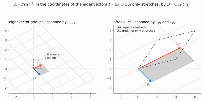
The eigenvectors give $A$ its natural coordinate grid. A cell spanned by $p_1, p_2$ is mapped to the cell spanned by $5p_1, 2p_2$: the same directions, only stretched. In these coordinates $A$ is the diagonal matrix $D = \operatorname{diag}(5, 2)$, which is what $A = PDP^{-1}$ says. In the standard grid the same map shears the unit square (dashed) into a slanted parallelogram. A defective matrix (e.g. the shear in Eigenvalue > Intuition) has too few eigen directions to build such a grid.

Write a start vector in the eigenbasis, $x_0 = c_1p_1 + c_2p_2$. Each application of $A$ multiplies the $p_1$-part by $5$ and the $p_2$-part by $2$, so $A^kx_0 = c_15^kp_1 + c_22^kp_2$. The $p_1$-part wins: the direction of $A^kx_0$ turns toward $p_1$, and the angle shrinks by about $\lambda_2/\lambda_1 = 2/5$ per step (right, log scale). This is power iteration, and the reason why the eigenvector of the largest eigenvalue dominates, e.g. in PageRank.

Sources#

• MML p. 105 (Def. 4.6, Def. 4.7 collinearity, non-uniqueness of eigenvectors)
• MML p. 106 (Def. 4.10 eigenspace, $E_\lambda = \ker(A - \lambda I)$), MML pp. 107–108 (Examples 4.5, 4.6, Def. 4.11 geometric multiplicity)
• MML pp. 111–112 (Thm. 4.12, Def. 4.13 defective, Thm. 4.15 spectral theorem, Example 4.8), MML pp. 113–114 (Example 4.9 PageRank)
• MML pp. 116–117 (Def. 4.19 diagonalizable, Thm. 4.20 eigendecomposition, Fig. 4.7)
• Use in MSI: spectral decomposition behind the eigenvalue test for PSD matrices