VL01 Introduction, Inverted Index, Zipf's Law
Course overview and organisation, keyword search with an inverted index and linear-time list intersection, tokenization, and Zipf's law of word frequencies.
Contents of the Course#
Two demos, both made in Freiburg (Slide 3):
- QLever, a graph database implementing the RDF and SPARQL standards (Lecture 6). RDF is a data model that is a variant of relational databases; SPARQL is its query language, a variant of SQL. See SPARQL and Knowledge Graphs.
- GRASP, a question answering system: an agentic AI, driven by a large language model, that interactively explores a graph database like a human would.
Research topics behind the demos, all covered in the course (Slide 4):
| Topic | Why |
|---|---|
| Indexing | needed for fast query times |
| Ranking | most relevant hits should come first |
| Databases | data stored in tables |
| Knowledge graphs | databases + interoperability |
| Error-tolerant search | errors in query or document |
| Web app stuff | HTTP, HTML, JavaScript, UTF-8 |
| Embeddings | use matrices and vectors |
| Vector databases and RAG | databases meet AI |
Keyword Search: Problem and Naive Solution#
For Exercise Sheet 1 the collection is 126,648 movie descriptions; queries have any number of keywords and at most three matching documents are returned. Ranking and documents that contain only some of the keywords follow in Lecture 2.
Naive solution (Slide 15): iterate over all documents and check each one, like grep. At about 1 GB/s this is fine for small collections, but not at web scale: Google indexes around pages; at about 10 kB of text per page that is about 10 PB TB GB of text.
Inverted Index#
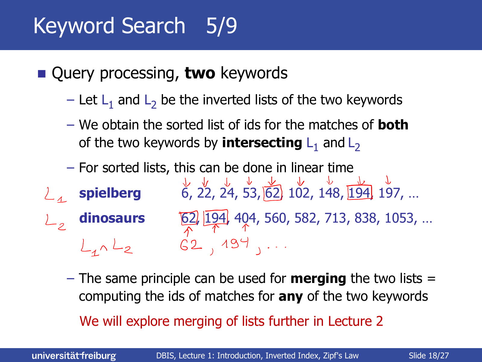
spielberg   6, 22, 24, 53, 62, 102, 148, 194, 197, …
dinosaurs   62, 194, 404, 560, 582, 713, 838, 1053, …
For Exercise Sheet 1, each inverted list contains a record ID at most once, even if the record contains the word several times. Alternative: store pairs (record ID, count), which Lecture 2 uses for ranking (term frequency).
See Inverted Index and Ranking for how this index is extended with scores.
Query Processing#
One keyword (Slide 17): the inverted list of the keyword already is the answer, i.e. the IDs of all records containing it.
Two keywords (Slide 18): let be the inverted lists of the two keywords. The sorted list of IDs that match both keywords is the intersection . For sorted lists this takes linear time with the zipper algorithm: keep one pointer per list, advance the pointer at the smaller ID, and output the ID when both pointers point to the same ID.
def intersect(l1: list[int], l2: list[int]) -> list[int]:
    """Zipper intersection of two sorted lists in time O(|l1| + |l2|)."""
    result, i, j = [], 0, 0
    while i < len(l1) and j < len(l2):
        if l1[i] < l2[j]:
            i += 1
        elif l1[i] > l2[j]:
            j += 1
        else:
            result.append(l1[i])
            i += 1
            j += 1
    return result
For the example,
The same principle merges the two lists, i.e. computes the IDs that match any of the two keywords (union); Lecture 2 uses merging with scores.
keywords (Slide 19): let be the inverted lists. Do a sequence of pairwise intersections (or merges): , then , and so on. Possible optimizations (not needed for the sheet):
- Order the lists such that . This minimizes the lengths of the intermediate results.
- -way intersect or merge in time .
Tokenization#
To build the index, the text has to be broken into words (Slide 20). Conceptually simple: define a set of word characters and a set of separator characters; words are the maximal sequences of word characters. For Exercise Sheet 1, a-z and A-Z are the word characters and everything else is a separator.
Construction of an Inverted Index#
Store the index in a map from strings (words) to arrays of ints (record IDs) (Slide 21). Construction algorithm:
- Iterate over all records, keeping track of the record ID.
- For each record, iterate over all the words it contains.
- For each word occurrence, append the ID of the current record to the word’s inverted list (create an empty list first if the word is new).
Since record IDs are visited in increasing order, every inverted list is automatically sorted. Code written in the lecture (public/code/lecture-01/inverted_index.py):
import re

class InvertedIndex:
    def __init__(self):
        self.inverted_lists: dict[str, list[int]] = {}

    def build_from_file(self, file_name: str):
        """
        >>> ii = InvertedIndex()
        >>> ii.build_from_file("example.tsv")
        >>> ii.inverted_lists
        {'a': [1, 2], 'movie': [1, 1, 3], 'film': [2]}
        """
        with open(file_name, "r") as file:
            record_id = 0
            for line in file:
                record_id += 1
                title, description, _ = line.split("\t", 2)
                words = re.findall(r"[A-Za-z]+", description)
                for word in words:
                    word = word.lower()
                    if word not in self.inverted_lists:
                        self.inverted_lists[word] = []
                    self.inverted_lists[word].append(record_id)
Zipf’s Law#
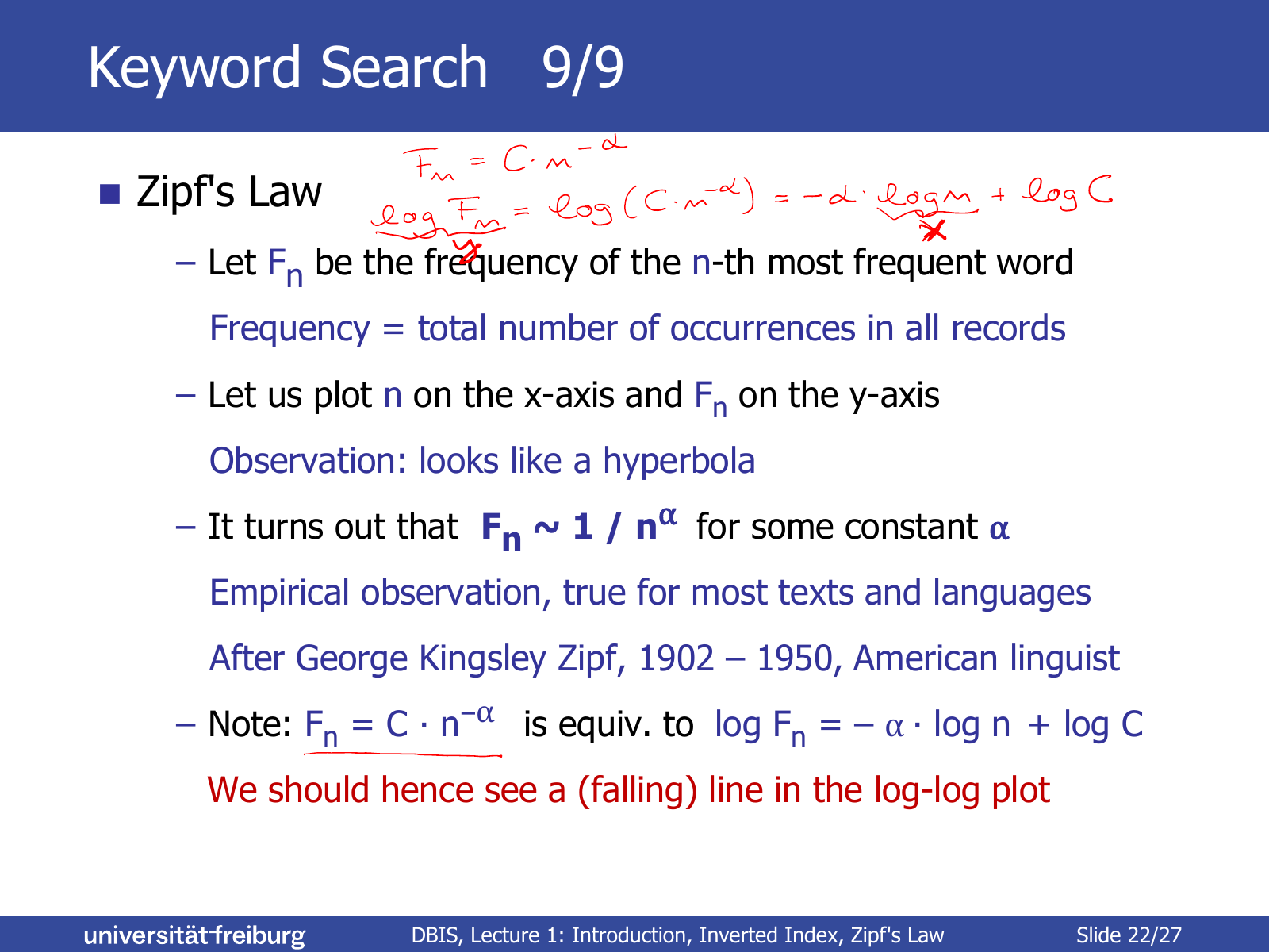
This is an empirical observation that holds for most texts and languages, named after George Kingsley Zipf (1902–1950, American linguist). Plotting on the x-axis against on the y-axis gives a curve that looks like a hyperbola. In words: there are only a few very frequent words, and most words are rare.
With a constant , is equivalent to
so in a log-log plot Zipf’s law shows up as a falling straight line with slope and intercept .
References#
Manning, Raghavan, Schütze: Introduction to Information Retrieval (online at informationretrieval.org); Wikipedia: Merge algorithm, Inverted index, Zipf’s law (Slide 27).
Concepts#
- Inverted Index — central data structure: word → sorted list of record IDs, built in one linear pass
- List Intersection — zipper algorithm intersects two sorted inverted lists in linear time (AND queries); merging gives OR queries
- Zipf’s Law — empirical power law of word frequencies, a line in the log-log plot
- Keyword Search — problem setting: return all documents containing all query keywords
- Tokenization — splitting text into maximal sequences of word characters
- K-way Merge — intersect/merge lists at once in