LectureDBISAI-written · not yet proofread

VL04 Query Planning Basics

The basic table operations projection, selection and Cartesian product, the translation of SELECT–FROM–WHERE queries into sequences of these operations, and simple cost estimates for choosing the cheapest sequence.

Held Tue 11 Nov 2025 Source lecture-04

Organisation#

Basic Operations#

From SQL queries to operations#

Lecture 3 explained by example what SELECT … FROM … WHERE … computes. An RDBMS computes it in three steps (Slide 5):

Internally, the RDBMS implements operations on tables (three today, more in Lecture 5).
A SQL query is translated into a sequence of these operations: query planning (done manually for ES4).
The sequence is executed: query processing (implemented in ES4).

The three basic operations are projection, selection and Cartesian product (“cross-product” is used synonymously). Each takes one or two tables as input and always outputs a single table (Slide 6).

Notation#

Recap from Lecture 3 (Relational Model, Slide 7): a table is a triple $T = (C, D, R)$ with column names $C = (c_1, \dots, c_k)$ , domains $D = (D_1, \dots, D_k)$ and a multiset $R$ of tuples $(r_1, \dots, r_k)$ with $r_j \in D_j$ . A tuple from $R$ is called a row, hence the letter $R$ .

Projection#

DefinitionProjection $\Pi_{\mathit{cols},\,\mathit{distinct}}(T)$ (Relational Algebra, Slide 9)

Signature: project(T, cols, distinct) or $\Pi_{\mathit{cols},\,\mathit{distinct}}(T)$ , where $T = (C, D, R)$ is a table with $k$ columns, $\mathit{cols} = (j_1, \dots, j_m)$ is a sequence of indices from $\{1, \dots, k\}$ , and $\mathit{distinct} \in \{\text{true}, \text{false}\}$ .

Result: the table $T' = (C', D', R')$ with

C' = (c_{j_1}, \dots, c_{j_m}), \quad D' = (D_{j_1}, \dots, D_{j_m}), \quad R' = \{(r_{j_1}, \dots, r_{j_m}) : r = (r_1, \dots, r_k) \in R\}.

If $\mathit{distinct}$ is true, all duplicates are removed from $R'$ (the multiset becomes the corresponding set).

Intuitively: keep a subset of the columns of a table.

ExampleProjection (Slide 10)

CREATE TABLE people(id TEXT, first TEXT, last TEXT);
SELECT DISTINCT first, last FROM people;

Operation: project(people, (2, 3), true).

id	first	last
Q36301	Anne	Hathaway
Q237251	Anne	Hathaway
Q106514	River	Phoenix
Q185140	Joaquin	Phoenix

Result: (Anne, Hathaway), (River, Phoenix), (Joaquin, Phoenix). The two Anne Hathaways collapse into one row because $\mathit{distinct}$ is true.

Selection#

Intuitively: filter the rows of a table by the predicate $\varphi$ .

Cartesian product#

Intuitively: all combinations of a row from $T_1$ with a row from $T_2$ .

ExampleCartesian product (Slide 14)

CREATE TABLE gender(id INT, what TEXT);
CREATE TABLE handed(id INT, what TEXT);
SELECT * FROM gender, handed;

gender has 3 rows (female, male, other) and handed has 2 rows (lefty, righty), so cartesian-product(gender, handed) has $2 + 2 = 4$ columns and $3 \cdot 2 = 6$ rows, one per (gender, handedness) pair.

Translating SQL into operations#

With project, select and cartesian-product, every query of the form (Slide 15)

SELECT [comma-separated list of column names]
FROM   [comma-separated list of tables]
WHERE  [Boolean expression on column names];

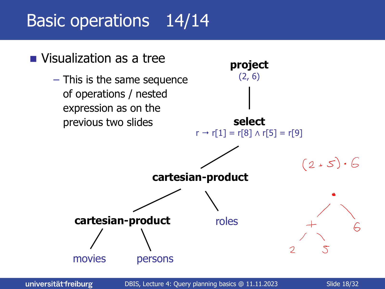
can be translated into a sequence of operations that computes its result: Cartesian product of the FROM tables, then selection with the WHERE expression, then projection onto the SELECT columns. This sequence can be written in three equivalent ways.

ExampleRunning example (Slides 16–18)

CREATE TABLE movies(id, title, year, score);
CREATE TABLE persons(id, name, birth_date);
CREATE TABLE roles(movie_id, person_id);

SELECT movies.title, persons.name
FROM movies, persons, roles
WHERE roles.person_id = persons.id AND roles.movie_id = movies.id;

Column indices after movies × persons × roles: 1 movies.id, 2 title, 3 year, 4 score, 5 persons.id, 6 name, 7 birth_date, 8 movie_id, 9 person_id.

As a sequence of operations:

T1 = cartesian-product(movies, persons)
T2 = cartesian-product(T1, roles)
T3 = select(T2, r → r[1] = r[8] ∧ r[5] = r[9])
T4 = project(T3, (2, 6), false)

As a single nested expression:

project(select(cartesian-product(cartesian-product(movies, persons), roles),
               r → r[1] = r[8] ∧ r[5] = r[9]), (2, 6))

This looks scary but is no harder to parse and evaluate than an arithmetic expression like $(((3 + 4) \cdot 4) - 3 + 8 \cdot 4) - 30 / 2$ .

In relational-algebra notation: $\Pi_{(2,6),\,\text{false}}\big(\sigma_{r[1] = r[8] \,\wedge\, r[5] = r[9]}((\text{movies} \times \text{persons}) \times \text{roles})\big)$ .

As a tree (leaves are the input tables, inner nodes the operations, the root produces the result):

Query Planning#

Motivation#

A single SQL query has many sequences of operations that compute its result. Regarding the result they are all equivalent (up to a permutation of the columns), but their processing time can differ greatly (Slide 19). Choosing a good sequence, a Query Plan, is query planning.

ExampleThree pairs of equivalent sequences (Slides 20–22)

Schemas: movies(id, title, year, score), persons(person_id, name, birth_date), roles(movie_id, person_id).

Example 1: SELECT * FROM movies, persons, roles;

Sequence 1: T1 = cartesian-product(movies, persons); T2 = cartesian-product(T1, roles)
Sequence 2: T1 = cartesian-product(movies, roles);   T2 = cartesian-product(T1, persons)

Example 2: SELECT * FROM movies, roles WHERE score >= 8.0;

Sequence 1: T1 = cartesian-product(movies, roles); T2 = select(T1, r → r[4] ≥ 8.0)
Sequence 2: T1 = select(movies, r → r[4] ≥ 8.0);  T2 = cartesian-product(T1, roles)

Example 3: SELECT DISTINCT title FROM movies, roles WHERE score >= 8.0;

Sequence 1: T1 = cartesian-product(movies, roles); T2 = select(T1, r → r[4] ≥ 8.0); T3 = project(T2, (2), true)
Sequence 2: T1 = select(movies, r → r[4] ≥ 8.0);  T2 = project(T1, (2), true)

Which sequence is better, assuming real data for the tables?

Cost and size estimates#

To pick a sequence (Slide 23):

estimate the cost of each operation in each sequence,
sum these to estimate the total cost of each sequence,
pick the sequence with the lowest total cost.

The cost of an operation depends on the size of its input, but input sizes are only known for the operations at the bottom of the tree (the actual tables). Each operation therefore also needs an estimate of the size of its result (rows and columns). Real query planners use even more statistics.

Let $T$ have $n$ rows and $k$ columns, $T_i$ have $n_i$ rows and $k_i$ columns, and let $k' = |\mathit{cols}|$ be the number of columns kept by a projection.

Operation	cost	rows	cols
$\Pi_{\mathit{cols},\,\mathit{distinct}}(T)$	$\sim n \cdot k'$	$\sim n$	$k'$
$\sigma_\varphi(T)$	$\sim n \cdot k$	$\sim n/2$	$k$
$T_1 \times T_2$	$\sim n_1 \cdot n_2 \cdot (k_1 + k_2)$	$n_1 \cdot n_2$	$k_1 + k_2$

Assumptions and reality check:

Projection (Slide 24): iterate over every row and copy the $k'$ selected columns. Reasonable if tables are stored in row order; in column order one could just copy “pointers” to the columns. The row estimate ignores duplicate removal for $\mathit{distinct} = \text{true}$ .
Selection (Slide 25): iterate over every row, $\varphi$ is evaluated in constant time and (rather arbitrarily) is true for half of the rows. Better: evaluate $\varphi$ on sample rows to estimate its cost and selectivity. If $\varphi$ has a special form (e.g. score ≥ 8.0) and the table is sorted by that column, not all rows need to be visited.
Cartesian product (Slide 26): these estimates are accurate, since the result of size $n_1 \cdot n_2 \cdot (k_1 + k_2)$ has to be produced anyway. Good query plans therefore avoid Cartesian products as far as possible; this leads to the join operations of Lecture 5.

Cost estimates for the examples#

Let movies have $n_1$ rows and 4 columns. In Example 1, persons has $n_2$ rows and 3 columns and roles has $n_3$ rows and 2 columns. In Examples 2 and 3, roles has $n_2$ rows and 2 columns. Handwritten annotations on Slides 27–29:

ExampleExample 1: order of Cartesian products (Slide 27)

Reasonable assumption: $n_1, n_2 \ll n_3$ (a movie has many actors, an actor plays in many movies).

	Operation	cost	rows	cols
Seq. 1	$T_1 = \text{movies} \times \text{persons}$	$7 n_1 n_2$	$n_1 n_2$	7
	$T_2 = T_1 \times \text{roles}$	$9 n_1 n_2 n_3$	$n_1 n_2 n_3$	9
Seq. 2	$T_1 = \text{movies} \times \text{roles}$	$6 n_1 n_3$	$n_1 n_3$	6
	$T_2 = T_1 \times \text{persons}$	$9 n_1 n_2 n_3$ (same as above)	$n_1 n_2 n_3$	9

The final product costs the same; Sequence 1 is better because $7 n_1 n_2 \ll 6 n_1 n_3$ . Combine the small tables first.

ExampleExample 2: select before product (Slide 28)

Assumption: $n_1 \ll n_2$ .

	Operation	cost	rows	cols
Seq. 1	$T_1 = \text{movies} \times \text{roles}$	$6 n_1 n_2$	$n_1 n_2$	6
	$T_2 = \sigma_\varphi(T_1)$	$6 n_1 n_2$	$n_1 n_2 / 2$	6
Seq. 2	$T_1 = \sigma_\varphi(\text{movies})$	$4 n_1$	$n_1 / 2$	4
	$T_2 = T_1 \times \text{roles}$	$\tfrac{n_1}{2} \cdot n_2 \cdot 6 = 3 n_1 n_2$	$n_1 n_2 / 2$	6

Totals: Sequence 1 $= 12\, n_1 n_2$ , Sequence 2 $= 3\, n_1 n_2 + 4 n_1$ , so Sequence 2 is better (push the selection below the product).

ExampleExample 3: select and project without the product (Slide 29)

Assumption: $n_1 \ll n_2$ .

	Operation	cost	rows	cols
Seq. 1	$T_1 = \text{movies} \times \text{roles}$	$6 n_1 n_2$	$n_1 n_2$	6
	$T_2 = \sigma_\varphi(T_1)$	$6 n_1 n_2$	$n_1 n_2 / 2$	6
	$T_3 = \Pi_{(2),\,\text{true}}(T_2)$	$n_1 n_2 / 2$	$n_1 n_2 / 2$	1
Seq. 2	$T_1 = \sigma_\varphi(\text{movies})$	$4 n_1$	$n_1 / 2$	4
	$T_2 = \Pi_{(2),\,\text{true}}(T_1)$	$n_1 / 2$	$n_1 / 2$	1

Totals: Sequence 1 $= 12.5\, n_1 n_2$ , Sequence 2 $= 4.5\, n_1$ , so Sequence 2 is better by a factor of order $n_2$ .

Query plans in SQLite3#

SQLite3 shows the plan it will use (Slide 30):

-- high-level description of the query plan
EXPLAIN QUERY PLAN
SELECT DISTINCT title FROM movies, roles WHERE score >= 8.0;

-- low-level execution plan
EXPLAIN
SELECT DISTINCT title FROM movies, roles WHERE score >= 8.0;

NoteScratchpad: optimal join order (material of Lecture 6)

The scratchpad links the Query Plan note under “Query planning”. Its content goes beyond this lecture and is covered in Lecture 6 (see Query Optimization):

A plan for $N$ tables combined by binary operations is a binary tree over them; the number of such trees grows like the Catalan numbers.
Join graph: one node per table, with an edge between $T_1$ and $T_2$ if they can be joined.
Cost model for joins: $\mathrm{size}(A \bowtie B) = \min\{\mathrm{size}(A), \mathrm{size}(B)\}$ and $\mathrm{cost}(A \bowtie B) = \mathrm{cost}(A) + \mathrm{cost}(B) + \mathrm{size}(A \bowtie B)$ .
The optimal cost of a set of tables $S$ is $\mathrm{cost}^*(S) = \min_{S_1, S_2} \{\mathrm{cost}^*(S_1) + \mathrm{cost}^*(S_2) + \mathrm{size}(S_1 \bowtie S_2)\}$ over all $S_1, S_2$ with $S_1 \cup S_2 = S$ , $S_1 \cap S_2 = \emptyset$ , $S_1, S_2 \neq \emptyset$ , and $\mathrm{cost}^* = 0$ for a single table. (The Lecture 6 slide writes the last term as $\mathrm{cost}^*(S_1 \bowtie S_2)$ ; by the cost function above, the join adds its result size.) The recursion is computed efficiently with dynamic programming, in rounds over subsets of increasing size.

Concepts#

Relational Algebra — formal definitions of projection $\Pi$ , selection $\sigma$ and Cartesian product $\times$ , with their cost and size estimates
Cartesian Product — all row combinations of two tables; $\#\mathrm{cols}$ add up, $\#\mathrm{rows}$ multiply, so plans avoid it
Query Plan — a sequence / nested expression / tree of operations computing a SQL query; choosing the cheapest one is query planning
Relational Model — the table definition $(C, D, R)$ on which the operations are defined
Cost model (query planning) — cost, rows and columns estimates per operation; total cost = sum over the sequence
Query processing — executing the chosen sequence of operations
EXPLAIN / EXPLAIN QUERY PLAN — inspecting SQLite3’s query plan