LectureDBISAI-written · not yet proofread

VL06 Indexing, Query Optimization, ACID

Index B+ trees for faster joins, computing the optimal join order of a query by dynamic programming over subsets of tables, and dynamic table updates with transactions and the ACID properties.

Held Tue 25 Nov 2025 Source lecture-06

Summary

An index B+ tree on a join column stores all (value, row index) pairs sorted in linked leaves below a search tree of degree $d$ , giving lookups in $O(\log n)$ time and $\log_d n$ IO operations. SQLite3 uses it for index-based joins and never for merge joins, although the leaves provide exactly the sorted input a merge join needs. The main part computes the optimal query plan for a set of binary joins: plans are parenthesised expressions, the joinable pairs are given by the join graph, and the optimal total cost $\text{cost}^*(S)$ satisfies a recursion over partitions of $S$ that is evaluated bottom-up in rounds (dynamic programming), because plain recursion is exponential like the naive Fibonacci recursion. Finally, SQL statements for changing tables, transactions and the four ACID properties are mentioned (not exam-relevant).

Organisation#

Index B+ tree#

Motivation (Slide 5). To accelerate a join, precompute an index on the join columns:

CREATE INDEX movies_index ON movies(movie_id);
CREATE INDEX persons_index ON persons(movie_id);

Measured in SQLite3 for a query like SELECT * FROM movies NATURAL JOIN roles;:

The join is faster with an index than without.
It is not faster with indexes on both join columns than with just one (explained by how SQLite3 joins, see Lookup below).

See Index B+ Tree.

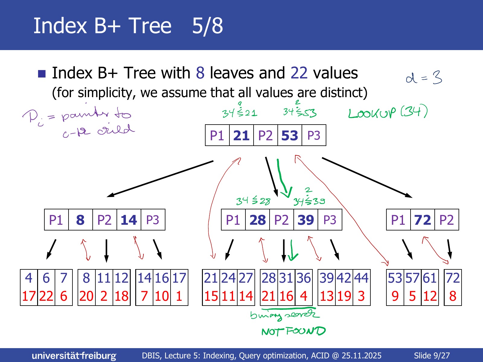
Joins in SQLite3. SQLite3 iterates over one join column and looks up each value in the B+ tree of the other join column. Hence an index on one join column suffices, which explains Observation 2 above.

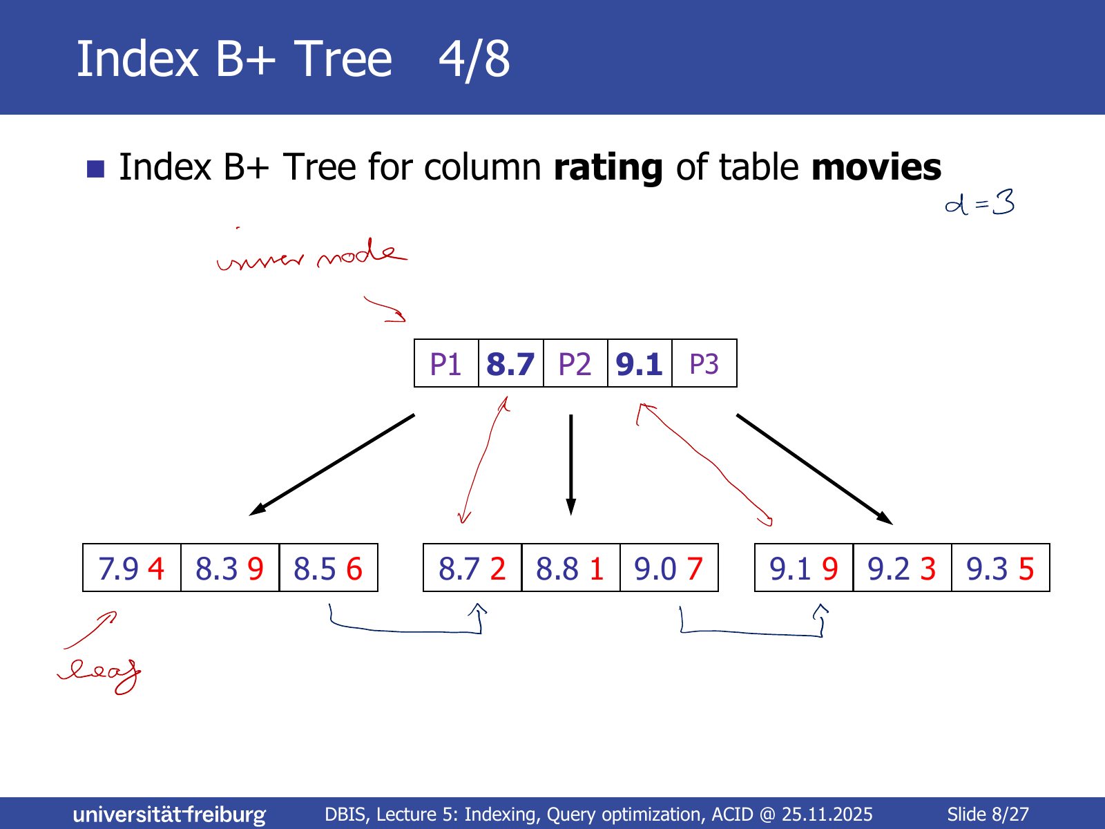
Iterating over the leaves (Slide 11). Scanning the linked leaves trivially yields all pairs (value, row index) in sorted order. With a B+ tree on both join columns, this is exactly the input of an efficient merge join (Lecture 5, Slide 13).

Variations (Slide 12)

A clustered B+ tree stores the full table rows in the leaves (instead of only the row index). The join result can then be produced directly from the tree, but it costs more space and is less IO-friendly.
A B tree (as opposed to a B+ tree) also stores full rows or (value, row index) pairs in the inner nodes. With one IO operation per inner node this reduces the number of children and hence increases the depth; also some data is stored twice (leaf and inner node).
In practice, updates of tables and indexes are important; the lecture only returns to updates of tables (see ACID below).

Computing the optimal query plan#

Recap (Slide 13). A query plan is a sequence of operations that computes the result table from the input tables. Its cost is estimated per operation from the size estimates of its inputs (Lectures 4 and 5, ES4 and ES5). Goal now: find the best plan among all possible plans automatically (Query Optimization).

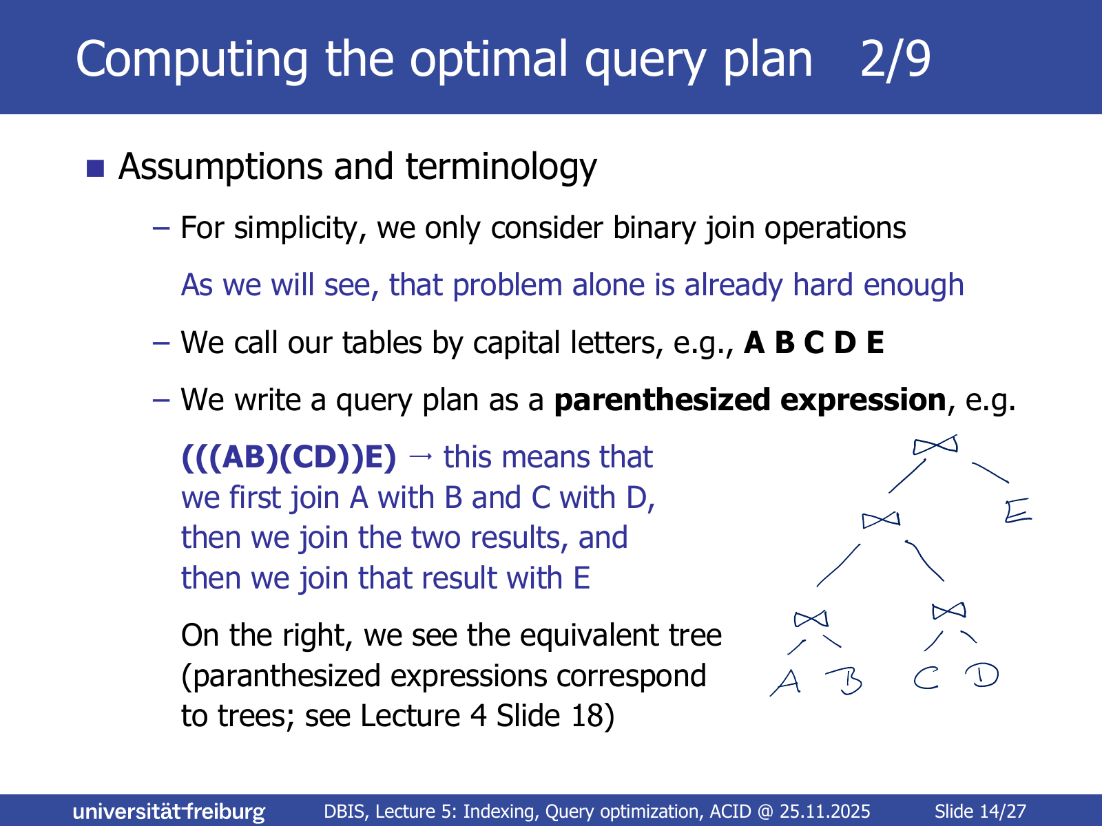
Assumptions and terminology (Slide 14)

Only binary join operations are considered; this problem alone is hard enough.
Tables are named by capital letters $A, B, C, D, E$ .
A query plan is written as a parenthesised expression, e.g. $(((AB)(CD))E)$ : first join $A$ with $B$ and $C$ with $D$ , then join the two results, then join that result with $E$ . Parenthesised expressions correspond to binary trees with tables as leaves and joins as inner nodes (Lecture 4, Slide 18).

ExampleJoin graph

SELECT title, name, role, award_name
FROM movies as A
NATURAL JOIN persons as B
NATURAL JOIN roles as C
NATURAL JOIN awards as D
NATURAL JOIN award_names as E

Adjacency lists (from the lecture): $A: C, D$ ; $B: C, D$ ; $C: A, B, D$ ; $D: A, B, C, E$ ; $E: D$ .

ExampleCost of plans for three tables (Slide 16)

$A$ : size 100, $B$ : size 200, $C$ : size 150, all with cost 0.

$\text{size}(AB) = \min\{100, 200\} = 100$ , $\text{cost}(AB) = 0 + 0 + 100 = 100$
$\text{size}((AB)C) = \min\{100, 150\} = 100$ , $\text{cost}((AB)C) = 100 + 0 + 100 = 200$
$\text{cost}(A(BC))$ : $\text{size}(BC) = 150 = \text{cost}(BC)$ , so $\text{cost} = 0 + 150 + \min\{100, 150\} = 250$
$\text{cost}((AC)B)$ : $\text{size}(AC) = 100 = \text{cost}(AC)$ , so $\text{cost} = 100 + 0 + \min\{100, 200\} = 200$

TheoremOptimal cost (Slide 17)

For a set $S$ of input tables, the cost of the optimal query plan is

\text{cost}^*(S) = \min_{\substack{S_1 \cap S_2 = \emptyset,\ S_1 \cup S_2 = S \\ S_1 \neq \emptyset,\ S_2 \neq \emptyset}} \big\{ \text{cost}^*(S_1) + \text{cost}^*(S_2) + \text{size}(S_1 \bowtie S_2) \big\},

with $\text{cost}^*(S) = 0$ for $|S| = 1$ . The recursion terminates because $S_1, S_2$ are strict subsets of $S$ . With the cost function above, $\text{size}(S_1 \bowtie S_2)$ is the minimum of the sizes of the tables in $S$ , independent of the plan. Only pairs $S_1, S_2$ that are joinable (see implementation details below) are considered.

A straightforward program evaluates this formula with a recursive function. This works badly, as the following interlude shows.

Interlude: Fibonacci numbers (Slide 18). $F(0) = 0$ , $F(1) = 1$ , $F(n) = F(n-1) + F(n-2)$ , i.e. $0, 1, 1, 2, 3, 5, 8, \dots$ The direct recursive function computes $F(30)$ reasonably fast, but $F(50)$ seems to take forever: its running time is $O(2^n)$ , because the same subproblems are recomputed over and over. Computing the values bottom-up, each from the two previous ones, takes linear time. The same idea (dynamic programming) applies to $\text{cost}^*$ .

ExampleOptimal plan for three tables (Slide 20)

$\text{size}(A) = 100$ , $\text{size}(B) = 200$ , $\text{size}(C) = 300$ ; every pair is joinable (the join graph is a clique).

Round	Plan	size	cost
1	$A$ / $B$ / $C$	100 / 200 / 300	0 / 0 / 0
2	$(AB)$	100	$0 + 0 + 100 = 100$
2	$(AC)$	100	$0 + 0 + 100 = 100$
2	$(BC)$	200	$0 + 0 + 200 = 200$
3	$((AB)C)$	100	$100 + 0 + 100 = 200$
3	$((AC)B)$	100	$100 + 0 + 100 = 200$
3	$(A(BC))$	100	$0 + 200 + 100 = 300$

$\text{cost}^*(\{A, B, C\}) = 200$ , attained by $((AB)C)$ and $((AC)B)$ : join the smallest table first.

Implementation details (Slide 21)

In round $k$ , do not iterate over all subsets of size $k$ ; only consider the combinations of plans from previous rounds whose union has size $k$ (already part of the algorithm above).
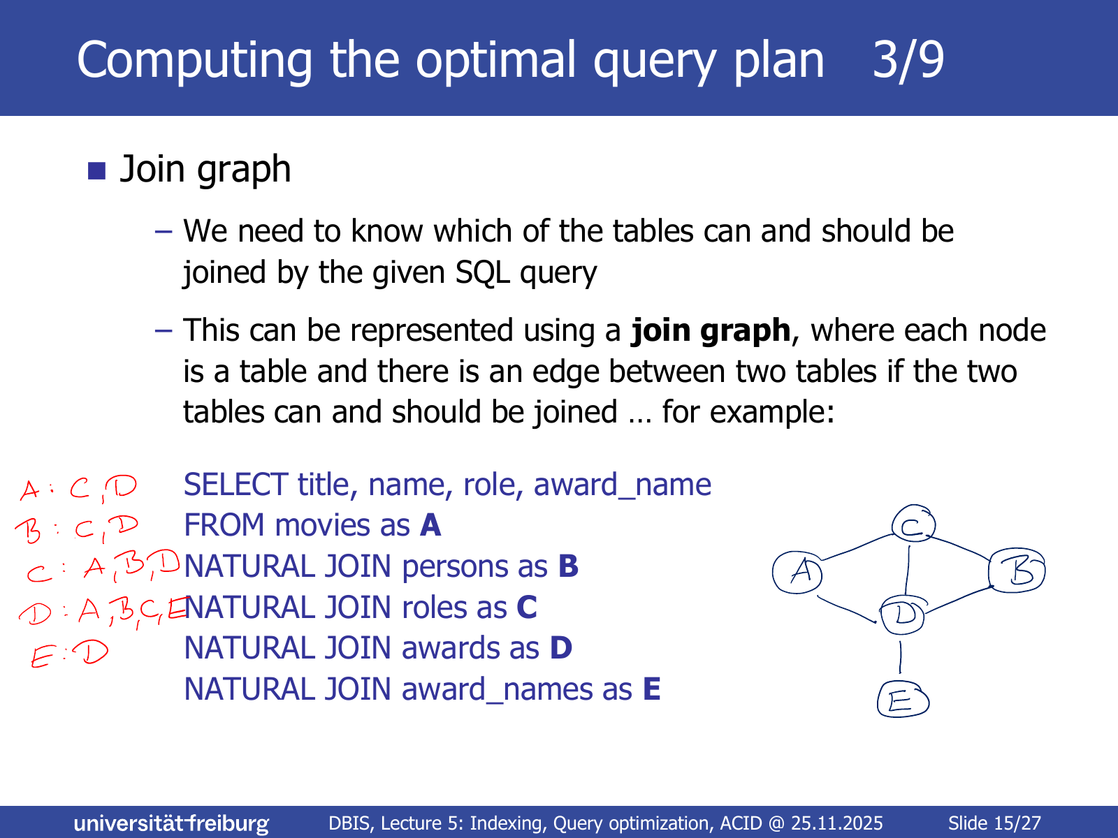
Two plans with table sets $S_1, S_2$ are joinable iff $S_1 \cap S_2 = \emptyset$ and the join graph has an edge between a table of $S_1$ and a table of $S_2$ .
The lecture code checks this with a nested loop in time $O(|S_1| \cdot |S_2|)$ ; in practice one uses bit masks.

# public/code/lecture-06/query-planning.py (excerpt)
for k in range(2, len(self.input_plans) + 1):
    optimal_plans[k] = {}
    for k1 in range(1, k // 2 + 1):
        k2 = k - k1
        for plan1 in optimal_plans[k1].values():
            for plan2 in optimal_plans[k2].values():
                if self.join_graph.joinable(plan1, plan2):
                    plan = QueryPlan.join(plan1, plan2)  # size = min, cost = c1 + c2 + size
                    if (plan.tables not in optimal_plans[k]
                            or plan.cost < optimal_plans[k][plan.tables].cost):
                        optimal_plans[k][plan.tables] = plan

ACID#

Dynamically changing tables (Slide 22). So far tables were read once and then only queried. This is a frequent use case (e.g. a new Wikidata dump once per month, for which one simply builds a new database). In many applications, however, the values change all the time: bank data (who has how much money), product data (which products at which price), HISinOne (who has which grade).

Changing rows (Slide 23):

CREATE TABLE movies(title TEXT, year INT, rating REAL);
INSERT INTO movies VALUES('Forrest Gump', 1994, 8.8);
UPDATE movies SET rating = 8.9 WHERE title = 'Inception';
DELETE FROM movies WHERE year < 2000;

Changing columns (Slide 24):

CREATE TABLE movies(title TEXT, year INT, score REAL);
ALTER TABLE movies ADD COLUMN genre;
ALTER TABLE movies DROP COLUMN genre;
ALTER TABLE movies RENAME COLUMN score TO rating;
ALTER TABLE movies ALTER COLUMN rating TYPE INT;

Transactions (Slide 25). With changing contents, errors become dangerous. In a read-only database a failed query just has to be asked again; but if in a money transfer from account $X$ to account $Y$ the amount was subtracted from $X$ but not added to $Y$ , the data is wrong.

See ACID Properties and https://en.wikipedia.org/wiki/ACID for an example of each.

References#

(Slide 27) Wikipedia: Database index, Query optimization, Dynamic programming, ACID. SQLite3: why there are no merge joins (https://www.sqlite.org/optoverview.html#hash_joins).

Open Questions#

How is an index B+ tree updated on INSERT/DELETE (keeping all leaves on one level and nodes at most $d$ entries)? The scratchpad’s “Updates” section is empty; Slide 12 announces updates, but the lecture only covers updates of table rows, not of the index.

Concepts#

Index B+ Tree — definition, lookup in $O(\log n)$ / $\log_d n$ IOs, use for joins in SQLite3, clustered B+ tree and B tree variants
Query Optimization — join graph, $\text{cost}^*(S)$ recursion and its dynamic-programming evaluation in rounds
Merge Join — equi-join of sorted join columns via a Zipper merge, fed by B+ tree leaves
Query Plan — plans as parenthesised expressions / binary trees with the total-cost function
Join — index-based join in SQLite3 and the merge join fed by B+ tree leaves
ACID Properties — atomicity, consistency, isolation, durability of transactions (not exam-relevant)
Join Graph — tables as nodes, edges between tables to be joined
Dynamic Programming — bottom-up evaluation of overlapping subproblems (Fibonacci, $\text{cost}^*$ )
Clustered B+ Tree — B+ tree with full rows in the leaves
B Tree — search tree with data also in inner nodes
Transaction — sequence of operations treated as one unit