LectureMSIAI-written · proofread

VL01 Introduction

What a model is and why we identify one, the notation used throughout the script, and the resistance estimation example in which three plausible estimators converge to three different values.

Script ch. 1.0–1.2Held Mon 19 Oct 2026 Source msi

1.0Introduction: Models and Why We Need Them#

The course aims to enable us to create models that help predict the behaviour of systems. The focus is on dynamic system models, i.e. systems that evolve over time (Script p. 9). A good model gives access to powerful engineering tools:

prediction of future behaviour (e.g. weather forecasting),
control and optimisation of technical systems, through feedback control or intelligent input design.

The course is about the process of obtaining such models. It builds on three fields: systems theory, statistics and optimisation.

Course roadmap (script):

Identification methods for static models and their statistical properties, with refreshers on statistics and optimisation (Part I–II).
Modelling of dynamic systems and identification of their parameters (Part III).

Model Predictive Control (MPC)#

1.1Mathematical Notation#

Source: Script pp. 9–10.

Sets, vectors, matrices#

Symbol	Meaning
$\mathbb{R}$ , $\mathbb{R}_+$ , $\mathbb{R}_{++}$	reals, non-negative reals, positive reals
$\mathbb{Z}$ , $\mathbb{N}$	integers, naturals including zero ( $\mathbb{N} = \mathbb{Z}_+$ )
$\mathbb{R}^n$ , $\mathbb{R}^{n\times m}$	vectors of dimension $n$ ; matrices with $n$ rows and $m$ columns
$\mathbb{S}^n$	symmetric matrices, $\{A \in \mathbb{R}^{n\times n} \mid A = A^\top\}$
$A \succcurlyeq 0$ , $A \succ 0$	$A \in \mathbb{S}^n$ positive semi-definite / positive definite (all eigenvalues $\geq 0$ / $> 0$ )
$A \succcurlyeq B$	matrix inequality: $A - B \succcurlyeq 0$

All vectors are column vectors by default: $\mathbb{R}^n = \mathbb{R}^{n\times 1}$ .
Concatenation: for $x \in \mathbb{R}^n$ , $y \in \mathbb{R}^m$ , $(x, y)$ is shorthand for $\begin{bmatrix} x \\ y \end{bmatrix} = [x^\top, y^\top]^\top \in \mathbb{R}^{n+m}$ .
Intervals: $[a,b]$ closed, $(a,b)$ open, $[a,b)$ half-open (contains $a$ , not $b$ ).

Norms#

$\|x\|$ : an arbitrary norm. $\|x\|_2$ : the Euclidean norm, $\|x\|_2^2 = x^\top x$ .
Weighted Euclidean norm with $Q \succ 0$ : $\|x\|_Q^2 = x^\top Q x$ .
$\|x\|_1 = \sum_{i=1}^n |x_i|$ , and $\|x\|_\infty = \max\{|x_1|, \dots, |x_n|\}$ .
Matrix norms are the induced operator norms unless stated otherwise. The Frobenius norm is $\|A\|_F^2 = \operatorname{trace}(AA^\top) = \sum_{i=1}^n \sum_{j=1}^m A_{ij}^2$ .

Derivatives#

For $f : \mathbb{R}^n \to \mathbb{R}^m$ :

With this convention the first-order Taylor expansion reads

f(x) = f(\bar x) + \nabla f(\bar x)^\top (x - \bar x) + o(\|x - \bar x\|).

Logic#

$A \Rightarrow B$ : “if $A$ then $B$ ”. $A \Leftrightarrow B$ : “ $A$ if and only if $B$ ”, also written “ $A$ iff $B$ ”.

Indices, time series and estimates#

Notation	Meaning
$x = [x_1, x_2, \dots, x_n]^\top$	components of $x \in \mathbb{R}^n$
$x_{1:N} \in \mathbb{R}^N$	a vector whose length grows with time, $x_{1:N} = [x_1, \dots, x_N]^\top$
$x^{[N]} \in \mathbb{R}^n$	a vector of fixed dimension that has been recursively updated up to time step $N$ (superscript in square brackets)
$\hat R$	an estimate of $R$
$R_\text{true}$	the true value of $R$
$\hat R_N$	the estimate of $R$ given the first $N$ measurements

1.2A Simple Example: Resistance Estimation#

Source: Script pp. 10–12, taken from Schoukens (2013).

Goal: estimate the resistance $R$ of a resistor from repeated measurements of current $i_k$ and voltage $u_k$ , $k = 1, \dots, N$ . The experiment is repeated to increase accuracy. Because of measurement noise, every pair $(u_k, i_k)$ is different.

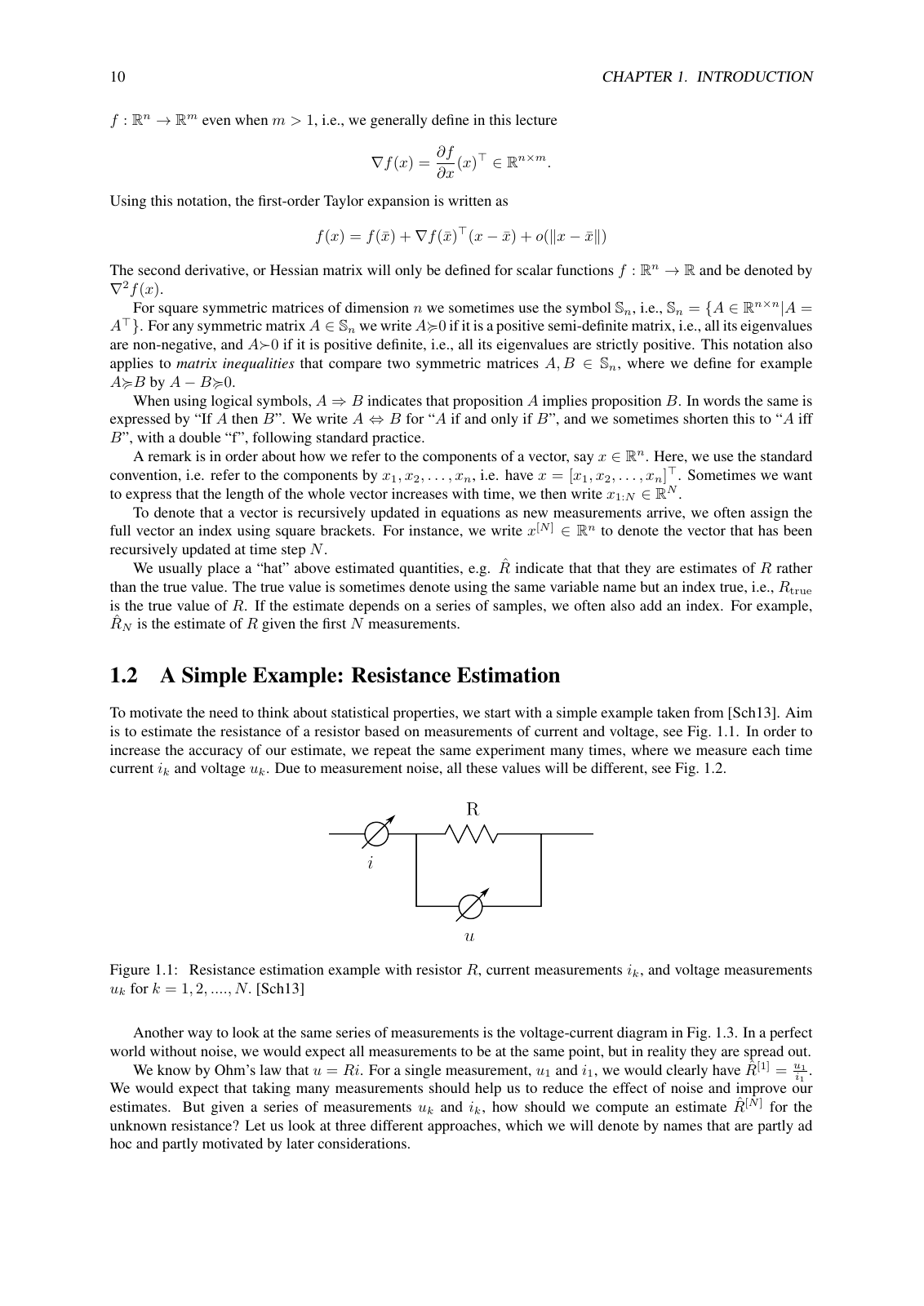
By Ohm’s law $u = Ri$ . A single measurement gives $\hat R^{[1]} = u_1 / i_1$ . Many measurements should reduce the effect of noise. The question is how to combine them.

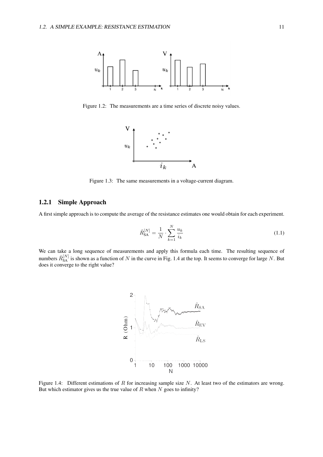
Fig. 1.2 shows the measurements as noisy time series. Fig. 1.3 shows them in the $u$ – $i$ plane: without noise all points would coincide, but in reality they are spread out.

1.2.1Simple Approach (SA)#

Average the single-measurement estimates:

\hat R^{[N]}_\text{SA} = \frac{1}{N} \sum_{k=1}^N \frac{u_k}{i_k} \tag{1.1}

As a function of $N$ it seems to converge (Fig. 1.4, top). But does it converge to the right value?

1.2.2Error-in-Variables (EV)#

First average voltages and currents separately, then divide:

\hat R^{[N]}_\text{EV} = \frac{\frac{1}{N}\sum_{k=1}^N u_k}{\frac{1}{N}\sum_{k=1}^N i_k} \tag{1.2}

The name comes from the estimator of the same name treated later. It also converges (Fig. 1.4, middle), but to a different value than SA.

1.2.3Least Squares (LS)#

Choose $R$ so that the model prediction $R\, i_k$ matches the measured voltage $u_k$ as well as possible in the squared sense:

\hat R^{[N]}_\text{LS} = \arg\min_{R \in \mathbb{R}} \sum_{k=1}^N (R\, i_k - u_k)^2 \tag{1.3}

\phantom{\hat R^{[N]}_\text{LS}} = \frac{\frac{1}{N}\sum_{k=1}^N u_k\, i_k}{\frac{1}{N}\sum_{k=1}^N i_k^2} \tag{1.4}

ProofDerivation of (1.4) (left as an exercise in the script)

Let $f(R) = \sum_{k=1}^N (R\, i_k - u_k)^2$ . Setting the derivative to zero:

f'(R) = 2 \sum_{k=1}^N (R\, i_k - u_k)\, i_k = 2\Big(R \sum_k i_k^2 - \sum_k u_k i_k\Big) \overset{!}{=} 0 \;\Longrightarrow\; R^* = \frac{\sum_k u_k i_k}{\sum_k i_k^2}.

Dividing numerator and denominator by $N$ gives (1.4). Since $f''(R) = 2\sum_k i_k^2 > 0$ (unless all $i_k = 0$ ), $f$ is strictly convex and $R^*$ is the unique minimiser.

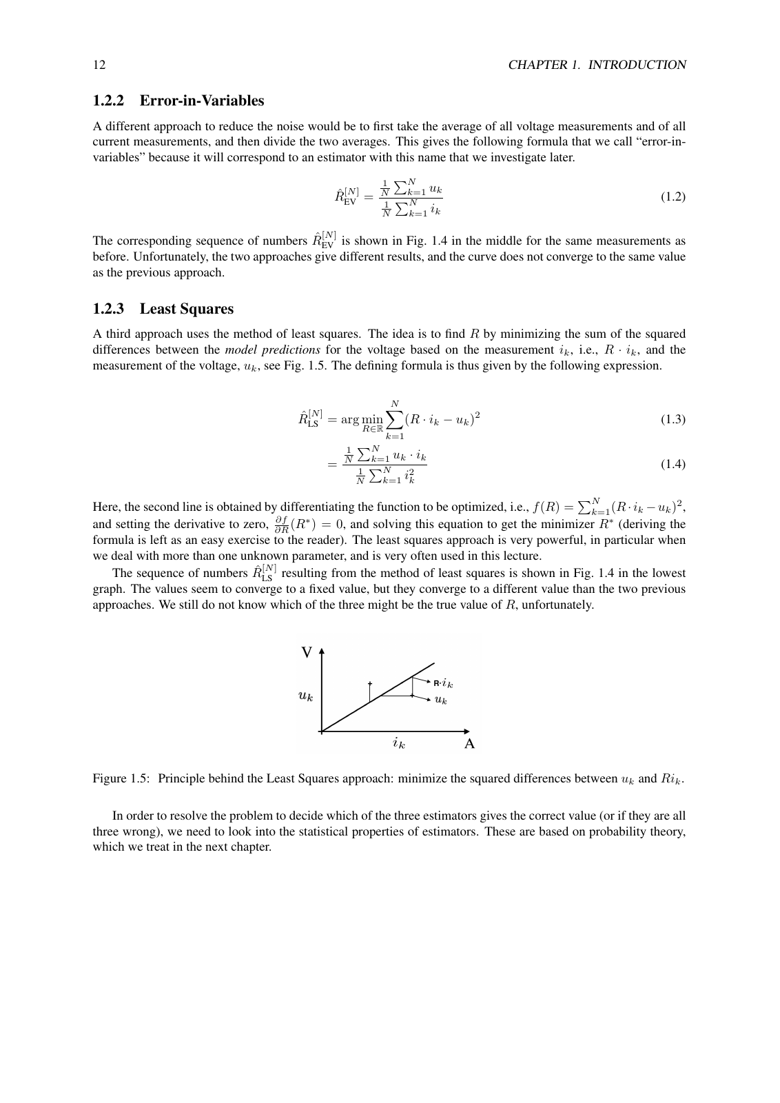
LS also converges (Fig. 1.4, bottom), but to yet another value. Least squares is very powerful, especially with more than one unknown parameter, and the course uses it constantly.

Takeaway#

Estimator	Formula	Combines the data by
SA	$\frac{1}{N}\sum_k \frac{u_k}{i_k}$	averaging the ratios
EV	$\frac{\sum_k u_k}{\sum_k i_k}$	taking the ratio of the averages
LS	$\frac{\sum_k u_k i_k}{\sum_k i_k^2}$	minimising the squared voltage residuals

All three look reasonable and all three converge as $N \to \infty$ , yet to three different limits. At least two of them must be wrong. Which one, if any, is correct cannot be decided by looking at the data. It requires the statistical properties of estimators, which are based on probability theory (Chapter 2).

NoteBeyond this lecture: resolved in Script §2.5

Model the data as $u_k = u_\text{true} + n_{u,k}$ and $i_k = i_\text{true} + n_{i,k}$ , with independent, zero-mean, i.i.d. noise of variances $\sigma_u^2, \sigma_i^2$ . Under this model EV is asymptotically unbiased: $\hat R_\text{EV}^{[N]} \to u_\text{true}/i_\text{true} = R_\text{true}$ . LS converges to $R_\text{true}\, \frac{i_\text{true}^2}{i_\text{true}^2 + \sigma_i^2}$ , so it underestimates $R$ whenever the current is noisy. SA is analysed separately and is also biased in general, since $\mathbb{E}\{u/i\} \neq \mathbb{E}\{u\}/\mathbb{E}\{i\}$ . See Script pp. 19–21.

Open Questions#

MPC vs. reinforcement learning, “online vs. offline”: which side is which? The usual framing is that MPC solves an optimisation online at every time step, while RL typically learns a policy offline. This isn’t in the script; check the recording.
Under what noise assumptions would LS be the right estimator? Presumably when only $u_k$ is noisy ( $\sigma_i = 0$ ); see Script §2.5.

Concepts#

Mathematical notation of the course: $\nabla f$ as transposed Jacobian, $x_{1:N}$ vs. $x^{[N]}$ , hat for estimates
Model / dynamic system model: what MSI wants to identify
Model Predictive Control: motivating application of models
Estimator: a rule mapping measurements to a parameter estimate
Resistance estimation example: running example comparing SA, EV and LS
Error-in-Variables estimator: ratio of averages
Least Squares estimator: minimiser of the sum of squared residuals