VL02 Probability and Statistics in a Nutshell

2.1Random Variables and Probabilities#

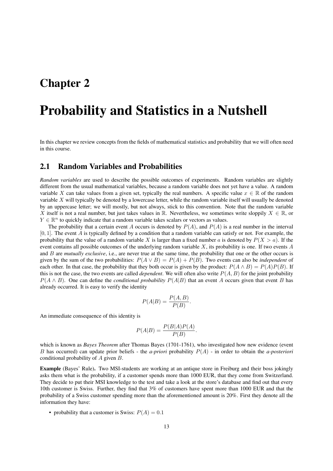
The section introduces a Random Variable $X$ as a description of an experiment’s outcomes. $X$ has no value itself and only takes values $x$. It then gives the rules for probabilities of events: the sum for mutually exclusive events and the product for independent events. From the Conditional Probability $P(A|B) = P(A,B)/P(B)$ it derives Bayes’ Theorem, which updates the a-priori $P(A)$ to the a-posteriori $P(A|B)$. The antique-store example turns $P(A) = 0.1$ into $P(A|B) = 2/3$ (Script pp. 13–14).

2.2Scalar Random Variables and Probability Density Functions#

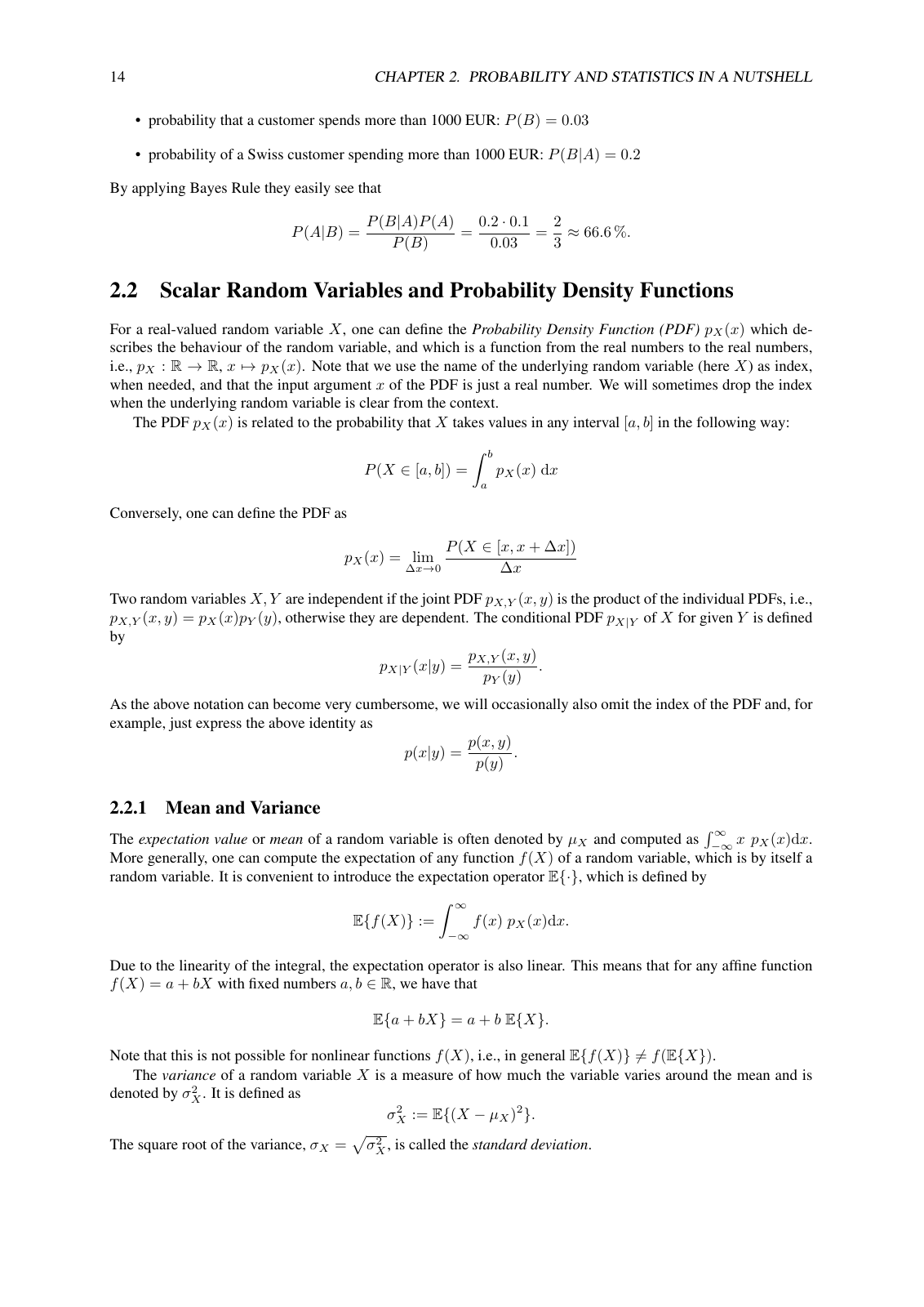
A real random variable is described by its Probability Density Function $p_X$. Probabilities are integrals of it, $P(X \in [a,b]) = \int_a^b p_X(x)\,\mathrm{d}x$. Independence and conditioning carry over from events to joint and conditional PDFs (Script p. 14).

2.2.1Mean and Variance#

The expectation operator $\mathbb{E}\{f(X)\} = \int f(x)\,p_X(x)\,\mathrm{d}x$ defines the mean (Expected Value) and the Variance $\sigma_X^2 = \mathbb{E}\{(X-\mu_X)^2\}$. The worked example shows $\sigma_X^2 = \mathbb{E}\{X^2\} - \mu_X^2$ (Script pp. 14–15).

2.2.2Simple Example: Uniform Distribution#

For the Uniform Distribution on $[a,b]$, integrating the PDF gives the mean $(a+b)/2$ and the variance $(b-a)^2/12$ (Script p. 15).

2.2.3The Normal Distribution#

The Normal Distribution $\mathcal{N}(\mu, \sigma^2)$ is named after its two parameters, which turn out to be exactly its mean and variance (Script p. 15).

2.2.4Covariance and Correlation#

Marginal PDFs come from integrating the joint PDF. The Covariance $\sigma(Y,Z)$ measures how $Y$ and $Z$ vary together, in the product of their units. The Correlation $\rho(Y,Z) = \sigma(Y,Z)/(\sigma_Y\sigma_Z)$ is its unitless version in $[-1,1]$ (Script pp. 15–16).

2.3Multidimensional Random Variables#

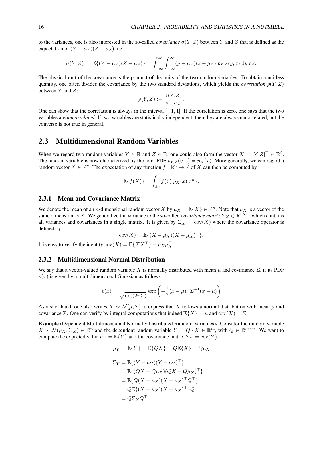
Stacking scalar random variables gives a random vector $X \in \mathbb{R}^n$ with a joint PDF. Expectations become integrals over $\mathbb{R}^n$ (Script p. 16).

2.3.1Mean and Covariance Matrix#

The mean $\mu_X \in \mathbb{R}^n$ is a vector. The variance generalises to the Covariance Matrix $\Sigma_X = \mathrm{cov}(X) = \mathbb{E}\{(X-\mu_X)(X-\mu_X)^\top\}$, which holds all variances and covariances. The vector analogue of §2.2.1 is $\mathrm{cov}(X) = \mathbb{E}\{XX^\top\} - \mu_X\mu_X^\top$ (Script p. 16). §2.3.2 (multidimensional normal distribution) follows in VL03.

Concepts#

• Random Variable: describes outcomes, takes values but has none
• Conditional Probability: $P(A|B) = P(A,B)/P(B)$, also for PDFs
• Statistical Independence: product rule for events and joint PDFs
• Bayes’ Theorem: a-priori → a-posteriori probability
• Probability Density Function: describes a scalar random variable, integrates to probabilities
• Expected Value: the expectation operator, linear for affine functions
• Variance: spread around the mean, $\sigma^2 = \mathbb{E}\{X^2\} - \mu^2$
• Uniform Distribution: first worked PDF example
• Normal Distribution: $\mathcal{N}(\mu, \sigma^2)$, parameters are mean and variance
• Covariance: joint variation of two variables
• Correlation: normalised covariance in $[-1, 1]$
• Covariance Matrix: all variances and covariances of a random vector